Tutorial: Running the pipeline • staRgate

Introduction

staRgate is an automated gating pipeline to process and analyze flow cytometry data to characterize the lineage, differentiation and functional states of T-cells.

This pipeline is designed to mimic the manual gating strategy of defining flow biomarker positive populations relative to a unimodal background population to include cells with varying intensities of marker expression. This is achieved via estimating the kernel density of the intensity distribution and corresponding derivatives. This pipeline integrates the density gating method in conjuction with some pre-processing steps achieved via the R package openCyto and an optional step with flowAI. The flow data is stored within R as a GatingSet object, which makes it easily transferable to other flow cytometry workflows available on BioConductor.

This vignette will walk through how to run the {staRgate} pipeline starting from importing an flow cytometry standard (FCS) file into R to preprocessing and gating, as well as identifying T-cell subpopulations for downstream analysis. This pipeline returns results at the single-cell level as well as the summarized sample-level data (for the percentages of positively expressing cells when identifying the subpopulations).

For illustration purposes, the example FCS file used in this vignette and stored in the package data is a concatenated file limited to the first 30k events/cells acquired to reduce the run time and file size.

After running {staRgate} to gate flow cytometry data, it is recommended to perform some quality checks (QC) on the gate placements to ensure they are reasonable. We suggest to use ridgeplots in addition to the ggcyto::autoplot to visualize the density distributions per marker across samples. When examining a large batch of samples, downsampling, such as to a random sample of 10k CD3+ cells, will make the QC process more manageable. In addition, random spot checks of a few samples would also be helpful QC to detect any edge cases.

Currently in this tutorial, we do not extend to the QC steps and suggest to lean on other examples for how to put together a ridgeplot for example. In the near future, we hope to incorporate some examples for the additional QC steps as well, stay tuned!

Installation

The {staRgate} package relies on a few Biocondcutor R packages. Before installing {staRgate}, first setup Bioconductor and install all dependencies.

Follow instructions here for installing Bioconductor

The essential dependencies for running the {staRgate} package include: flowCore, and flowWorkspace.

The following packages are needed to fully run the pipeline as shown in this Tutorial, but not required for the {staRgate} code chunks to run: openCyto, ggplot2, ggcyto, gt

# Load libraries
library(staRgate)
library(openCyto)
library(flowWorkspace)
#> As part of improvements to flowWorkspace, some behavior of
#> GatingSet objects has changed. For details, please read the section
#> titled "The cytoframe and cytoset classes" in the package vignette:
#> 
#>   vignette("flowWorkspace-Introduction", "flowWorkspace")
library(flowCore)
# Just for plotting in the vignette
library(ggplot2)
library(ggcyto)
#> Loading required package: ncdfFlow
#> Loading required package: BH

# Set up dynamic variables
pt_samp_nm <- "flow_sample_1"

## File path to the FCS file
path_fcs <- system.file("extdata", "example_fcs.fcs", package = "staRgate", mustWork = TRUE)

## File path to the compensation matrix csv file
## Expect format to match flowJo exported version
path_comp_mat <- system.file("extdata", "comp_mat_example_fcs.csv", package = "staRgate", mustWork = TRUE)

## File path for outputs/saving
# Maybe not the best sol, but create a temp dir?
path_out <- tempdir()
# Print the path_out for user to see
path_out
#> [1] "/tmp/RtmprmwtZO"

## File path Gating template
gtFile <- system.file("extdata", "gating_template_x50_tcell.csv", package = "staRgate", mustWork = TRUE)

## File path to biexp parameters
## Expects 4 columns: full_name, ext_neg_dec, width_basis, positive_dec
## full name should contain the channel/dye name
# 3 remaining cols fill in with desired parameter values
path_biexp_params <- system.file("extdata", "biexp_transf_parameters_x50.csv", package = "staRgate", mustWork = TRUE)

## File path to positive peak thresholds
path_pos_peak_thresholds <- system.file("extdata", "pos_peak_thresholds.csv", package = "staRgate", mustWork = TRUE)

Input files and function parameters

In order to run the pipeline, the user must have the data in flow cytometry standard (FCS) format. This is usually the output from flowJo. All of these input files except the bin size are expected to be comma-separated values (csv) files. Please see the inst folder of the package for examples of the formats.

Compensation matrix from manual gating-
- Matrix where the column and row names correspond to the channel names, cell values correspond to the spillover correction to be applied.
- This can be exported as a csv in flowJo’s options
Biexponential transformation parameters-
- This is a table specifying the parameters (negative decades, width basis and positive decades) to be applied to the listed channels
Gating template
- A gating template is required to run the pre-gating via openCyto
- The package includes a gating template tailored for gating this panel of T-cell markers.
- For examples of how to modify the gating template, please refer to the openCyto documentation.
Bin size
- From a systematic grid search, we have found bin sizes of 40 to 50 works well for the density gating

A few things to keep in mind when debugging/iterating through gating:

If saving at the same path with same name (i.e., rerunning the same code), the GatingSet folder from the flowWorkspace::save_gs() command needs to be deleted for openCyto to save again, otherwise, will encounter an error related to an invalid path from the flowWorkspace::save_gs() function

Example

Below is an example of gating 1 FCS sample.

Import FCS

# Read in gating template
dtTemplate <- data.table::fread(gtFile)

# Load the FCS
gt_tcell <- openCyto::gatingTemplate(gtFile)
#> expanding pop: -/++/-
#> Adding population:fsc_ssc_qc
#> Adding population:nonDebris
#> Adding population:singlets
#> Adding population:cd14-cd19-
#> Adding population:live
#> Adding population:cd3
#> Adding population:cd4+
#> Adding population:cd8+
#> Adding population:cd4+cd8+
#> Adding population:cd4-cd8+
#> Adding population:cd4+cd8-
#> Adding population:cd4-cd8-

cs <- flowWorkspace::load_cytoset_from_fcs(path_fcs)

# Create a GatingSet of 1 sample
gs <- flowWorkspace::GatingSet(cs)

# Check- how many cells is in the FCS file?
n_root <- flowWorkspace::gh_pop_get_count(gs, "root")

# The example FCS has 30000 cells
n_root
#> [1] 30000

Compensation

# Apply comp
gs <- getCompGS(gs, path_comp_mat = path_comp_mat)

# Can check that the comp was applied
chk_cm <- flowWorkspace::gh_get_compensations(gs)

# Not aware of an accessor that we can use for this
head(methods::slot(chk_cm, "spillover"), 2)
#>          AF700-A     APC-A APC-f750-A      BB515-A    BB660-A    BB700-A
#> AF700-A 1.000000 0.0248301  0.2492840  0.009679220 0.00268438 0.04732480
#> APC-A   0.132334 1.0000000  0.0337338 -0.000160633 0.01598550 0.00443383
#>            BB790-A    BUV395-A     BUV496-A     BUV563-A   BUV615-A   BUV661-A
#> AF700-A 0.01730770 0.001813870  1.81722e-03  1.45041e-03 0.00249455 0.00220337
#> APC-A   0.00122597 0.000471851 -5.18352e-05 -3.25396e-05 0.00127167 0.11436300
#>          BUV737-A   BUV805-A      BV421-A     BV480-A     BV510-A     BV570-A
#> AF700-A 0.1387160 0.03310420  5.11994e-05 0.003390200 2.60901e-03 2.45899e-03
#> APC-A   0.0221613 0.00527436 -4.09868e-04 0.000113668 4.37466e-05 5.85607e-05
#>            BV605-A    BV650-A   BV711-A    BV750-A    BV786-A        PE-A
#> AF700-A 0.00358515 0.00445768 0.2127300 0.08483990 0.04394760 0.006840740
#> APC-A   0.00085079 0.13844100 0.0285134 0.00973321 0.00417643 0.000280757
#>         PE-CF594-A  PE-Cy5-A PE-Cy5.5-A  PE-Cy7-A
#> AF700-A 0.02926360 0.0164829  0.3260510 0.1032330
#> APC-A   0.00541964 0.2677470  0.0810869 0.0215633

Transformation

The transformation applied to all channels is the same: biexponential with extra negative decades = 0.5, positive decades = 4.5 and width basis = -30

The structure of the table of parameters (as .csv format) should be first column for the flurochrome names corresponding to the panel, followed by the parameters.

tbl_biexp_params <-
  utils::read.csv(path_biexp_params) |>
  janitor::clean_names(case="all_caps")

head(tbl_biexp_params, 2)
#>   FULL_NAME EXT_NEG_DEC WIDTH_BASIS POSITIVE_DEC
#> 1  BUV395-A         0.5         -30          4.5
#> 2  BUV496-A         0.5         -30          4.5

Currently, the package only supports biexponetial transformation for all channels with the getBiexpTransformGS() function. However, the user may choose to create a transformation list explicitly if other transformations (e.g., archsin) are desired.

Note that the flowWorkspace package also allows for an automated transformation calculation “guessing” appropriate parameters. We chose to explicitly specify the biexponential transformation with fixed parameters for all channels to match the manual gating strategy used in flowJo for a more direct comparison of {staRgate} when benchmarking against the manual gating results.

# Save the pre-transformed data to compare ranges 
# And check that transformation was applied
dat_pre_transform <-
  flowWorkspace::gh_pop_get_data(gs) |>
  flowCore::exprs()

# Apply biexp trans
gs <- getBiexpTransformGS(gs, path_biexp_params = path_biexp_params)

## **Optional**-- to check what pre-transformed data against post
# save the post-transformed data
dat_post_transform <-
  flowWorkspace::gh_pop_get_data(gs) |>
  flowCore::exprs()

## **Optional**-- to check that the transformation worked on all provided channels!
## Commented out for ease of length 
# summary(dat_pre_transform)
# summary(dat_post_transform)

Pre-gating

In this context, pre-gating is defined as gating from the root population (all cells acquired) up to key parent populations: CD3+, or CD4+/CD8+ subsets. Then we will gate each marker indpendently.

The flowAI step serves as a quality control (QC) to match the first Time gate step that is typically done in manual gating. It is possible, however, that the user may choose to skip this step if flowAI excludes too many cells.

The first step of the gating template is a QC step that is especially important to include if the user chooses to exclude the flowAI step.

In this tutorial, we will skip the flowAI step to ease the length.

# Pre-gating up to CD4/8+ with `r BiocStyle::Biocpkg("openCyto")`
## Set seed using today's date
set.seed(glue::glue({
  format(Sys.Date(), format = "%Y%m%d")
}))

openCyto::gt_gating(gt_tcell, gs)
#> Gating for 'fsc_ssc_qc'
#> done!
#> done.
#> Gating for 'nonDebris'
#> done!
#> done.
#> Gating for 'singlets'
#> done!
#> done.
#> Gating for 'cd14-cd19-'
#> done!
#> done.
#> Gating for 'live'
#> done!
#> done.
#> Gating for 'cd3'
#> done!
#> done.
#> Gating for 'cd8+'
#> done!
#> done.
#> Gating for 'cd4+'
#> done!
#> done.
#> Population 'cd4-cd8-'
#> done.
#> Population 'cd4+cd8-'
#> done.
#> Population 'cd4-cd8+'
#> done.
#> Population 'cd4+cd8+'
#> done.
#> finished.

## Check autoplot
ggcyto::autoplot(gs[[1]])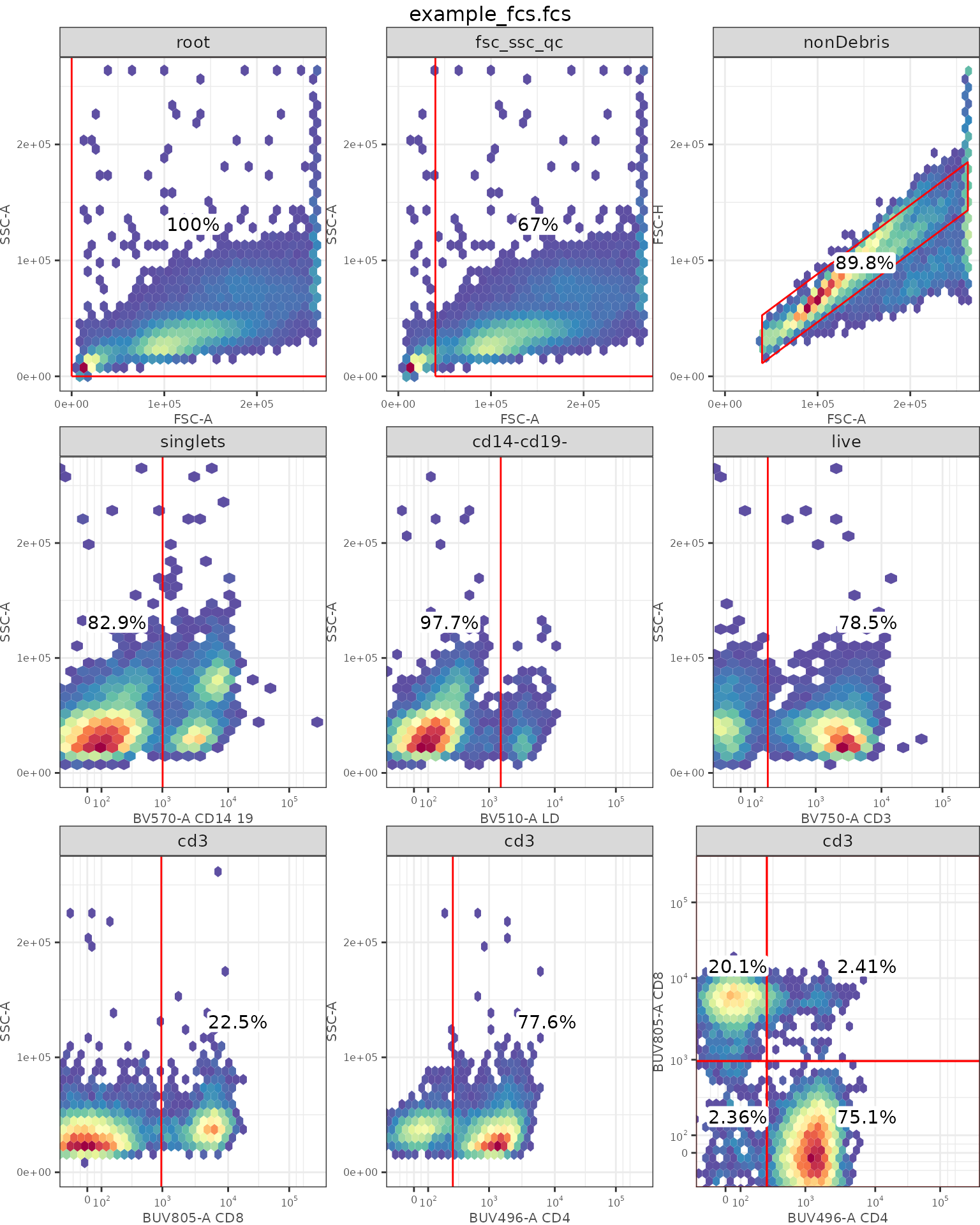

Extract intensity matrix

Grab the channel and marker names in the gs object

When extracting intensity_matrix, it is labeled with the channel names rather than the marker names.
The marker_chnl_names mapping created below will be used to rename the column names to the marker names, which will make calling the appropriate columns easier when analyzing the data

## Grab marker names from GatingSet for labeling col names in intensity matrix
## Can skip this step if you know the names of the channels that correspond to your marker names in your FCS files
# In that case, supply strings for `chnl` and `marker_full` is fine. Such as:
# chnl = c("BV750-A", "BUV496-A")
# marker_full = c("CD3", "CD4)

# This returns a named character vector
# With the channel names as names and marker names as the values
marker_chnl_names <- flowWorkspace::markernames(flowWorkspace::gh_pop_get_data(gs))

## Specify which markers to gate based on individual density distributions
# For our Tcell panel, we only want to apply the density gating on
# these 23 markers
markers_to_gate = c("CD45RA", "ICOS", "CD25", "TIM3", 
                    "CD27", "CD57", "CXCR5", "CCR4", 
                    "CCR7", "HLADR", "CD28", "PD1", 
                    "LAG3", "CD127", "CD38", "TIGIT", 
                    "EOMES", "CTLA4", "FOX_P3", "GITR",
                    "TBET", "KI67", "GZM_B")

Next we grab the intensity values and indicators for the pre-gating steps.

# Extract intensity matrix from GatingSet object
## Grab the intensity matrix from GatingSet
intensity_dat <-
  cbind(
    # This grabs the intensity matrix with intensity values
    flowWorkspace::gh_pop_get_data(gs) |>
      flowCore::exprs(),
    # the gh_pop_get_indices grabs the 0/1 for whether gated as pos/neg 
    # for each step specified
    "fsc_ssc_qc" = flowWorkspace::gh_pop_get_indices(gs, y = "fsc_ssc_qc"),
    "nonDebris" = flowWorkspace::gh_pop_get_indices(gs, y = "nonDebris"),
    "singlets" = flowWorkspace::gh_pop_get_indices(gs, y = "singlets"),
    "cd14_neg_19_neg" = flowWorkspace::gh_pop_get_indices(gs, y = "cd14-cd19-"),
    "live" = flowWorkspace::gh_pop_get_indices(gs, y = "live"),
    "cd3_pos" = flowWorkspace::gh_pop_get_indices(gs, y = "cd3"),
    "cd4_pos" = flowWorkspace::gh_pop_get_indices(gs, y = "cd4+"),
    "cd8_pos" = flowWorkspace::gh_pop_get_indices(gs, y = "cd8+")
  ) |>
  # The intensity matrix is a matrix object. Convert to tibble.
  tibble::as_tibble() |>
  # Rename with colnames which are the channel names
  # to marker names because it's easier to call columns by markers
  # Rename using the marker_chnl_names we created above
  # But we need it flipped when supplying to dplyr::rename()
  # Where the names = value to rename to (marker names) 
  # The values of the vector = current names (Channel names)
  dplyr::rename(
    stats::setNames(names(marker_chnl_names),
                    # Clean up the marker names, make them all caps
                    janitor::make_clean_names(marker_chnl_names, 
                                              case = "all_caps", 
                                              replace = c("-" = "", "_" = "", " " = "")))
                ) |>
  dplyr::mutate(
    # Create a 4-level category for cd4, cd8 neg/pos
    # in order to calculate the percentages individually within these parent populations
    cd4_pos_cd8_pos = dplyr::case_when(
      cd3_pos == 1 & cd4_pos == 1 & cd8_pos == 1 ~ "cd4_pos_cd8_pos",
      cd3_pos == 1 & cd4_pos == 1 & cd8_pos == 0 ~ "cd4_pos_cd8_neg",
      cd3_pos == 1 & cd4_pos == 0 & cd8_pos == 1 ~ "cd4_neg_cd8_pos",
      cd3_pos == 1 & cd4_pos == 0 & cd8_pos == 0 ~ "cd4_neg_cd8_neg"
    )
  )

## Preview of intensity matrix
head(intensity_dat, 2)
#> # A tibble: 2 × 44
#>   `FSC-A` `FSC-H` `FSC-W` `SSC-A` `SSC-H` `SSC-W`  KI67  TBET GZM_B   PD1  LAG3
#>     <dbl>   <dbl>   <dbl>   <dbl>   <dbl>   <dbl> <dbl> <dbl> <dbl> <dbl> <dbl>
#> 1  14579.  12925.  91156.   6783.   6899.  59440.  898.  995.  949.  922. 1184.
#> 2  47535.  36802. 124831.  21010.  20507.  79210.  732. 1178.  775.  914. 1169.
#> # ℹ 33 more variables: CD127 <dbl>, CD38 <dbl>, CD45RA <dbl>, CD4 <dbl>,
#> #   ICOS <dbl>, CD25 <dbl>, TIM3 <dbl>, CD27 <dbl>, CD8 <dbl>, CD57 <dbl>,
#> #   CXCR5 <dbl>, LD <dbl>, CD1419 <dbl>, CCR4 <dbl>, CCR7 <dbl>, HLADR <dbl>,
#> #   CD3 <dbl>, CD28 <dbl>, TIGIT <dbl>, EOMES <dbl>, CTLA4 <dbl>, FOX_P3 <dbl>,
#> #   GITR <dbl>, Time <dbl>, fsc_ssc_qc <dbl>, nonDebris <dbl>, singlets <dbl>,
#> #   cd14_neg_19_neg <dbl>, live <dbl>, cd3_pos <dbl>, cd4_pos <dbl>,
#> #   cd8_pos <dbl>, cd4_pos_cd8_pos <chr>

Gating on T-cell subsets

Pseudo-negative control

For this T-cell panel, we recommend using the CD3- cells as a pseudo-negative control when gating CD127 and CD28 as these two markers are expected to be predominantly negatively-expressing on CD3- cells. This mimics the isotype-based gating approach. Here we recommend using the 95th percentile of the CD3- distributions.

To ensure we only capture the CD3- cells, we first filter to the live cells then to cd3_pos == 0

gates_pseudo_neg = 
  dplyr::filter(intensity_dat, live == 1, cd3_pos == 0) |>
  dplyr::select(CD127, CD28) |>
  dplyr::summarise(
    dplyr::across(c(CD127, CD28),
                  ~ quantile(.x, 0.95))
  )

Empirical gating

For the other functional and differentiation markers where we cannot borrow CD3- as the pseudo-negative control, we gate empirically based on the CD3+ density distribution per marker.

The suggested strategy is based on all CD3+, but this can be customized based on the string corresponding to the column name supplied to subset_col in the get_density_gates function
The suggested number of bins for density estimation is 40 as some level of smoothing is required to reduce the noise and picking up false peaks.
When multiple samples from the same batch or experiment run (e.g., samples are processed on the same day), we recommend to borrow information from other samples by pooling all CD3+ across the same batch before applying the density gating.
If interested in pooling across experiment runs, consider visualizing for any batch-level intensity shifts and variations before pooling samples together.

For illustration purposes, we will only apply density gating on a few markers.

# Density gating parameters
# peak detection ratio where any peak < 1/10 of the tallest peak will be 
# considered as noise
peak_r <- 10 
# smoothing to apply to the density estimation
# Using the default of 512 creates many little bumps/noise that are artifacts 
# From a systematic grid search, we found the bin sizes of ~40-50 works best
bin_i <- 40

# Remove any very negative values that are artifacts from autogating
# -1000 on the biexp transformed scale corresponds to roughly -3300 on the original
# intensity scale so this is quite conservative.
neg_intensity_thres <- -1000

# select a few markers to gate
example_markers <- c("LAG3", "CCR7", "CD45RA")

# Read in positive peak thresholds
pos_thres <- utils::read.csv(path_pos_peak_thresholds) |>
  janitor::clean_names(case = "all_caps")

# calculate the gates
dens_gates_pre <-
  dplyr::filter(intensity_dat, cd3_pos == 1) |>
  getDensityGates(
    intens_dat = _,
    marker = example_markers,
    subset_col = "cd3_pos",
    bin_n = bin_i,
    peak_detect_ratio = peak_r,
    pos_peak_threshold = pos_thres,
    neg_intensity_threshold = neg_intensity_thres
  )

# Since we apply density gating on CD3+ cells but
# Would like to calculate subpopulations with CD4+ and CD8+ as
# the starting parent population, we need to add corresponding rows
# to pass into getGatedDat()
dens_gates <-
  # Stack the pseudo-neg gated markers and empirically gated markers
  dplyr::bind_cols(dens_gates_pre, gates_pseudo_neg) |>
  tibble::add_row() |>
  tibble::add_row() |>
  tibble::add_row() |>
  dplyr::mutate(cd4_pos_cd8_pos = c("cd4_neg_cd8_neg", "cd4_pos_cd8_neg", "cd4_neg_cd8_pos", "cd4_pos_cd8_pos")) |>
  tidyr::fill(-cd4_pos_cd8_pos, .direction = "down")

# View updated gates with the col for CD4/CD8
dens_gates
#> # A tibble: 4 × 7
#>   cd3_pos  LAG3  CCR7 CD45RA CD127  CD28 cd4_pos_cd8_pos
#>     <dbl> <dbl> <dbl>  <dbl> <dbl> <dbl> <chr>          
#> 1       1 1634. 1768.  1486. 1327. 1251. cd4_neg_cd8_neg
#> 2       1 1634. 1768.  1486. 1327. 1251. cd4_pos_cd8_neg
#> 3       1 1634. 1768.  1486. 1327. 1251. cd4_neg_cd8_pos
#> 4       1 1634. 1768.  1486. 1327. 1251. cd4_pos_cd8_pos

# get indicator col
example_intensity_gated <-
  getGatedDat(
    # Only gate T-cells, which are CD3+ 
    dplyr::filter(intensity_dat, cd3_pos == 1),
    subset_col = "cd4_pos_cd8_pos",
    cutoffs = dens_gates
  )

Visualizing the gates

LAG3 for all CD3+

# Plot the gate for visual
intensity_dat |>
  dplyr::filter(cd3_pos == 1) |>
  # additional step to remove large intensity values only when density gating.
  # Still kept in the data
  dplyr::filter(!(dplyr::if_any(dplyr::all_of(markers_to_gate), ~ .x < neg_intensity_thres))) |>
  ggplot() +
  geom_density(aes(LAG3)) +
  geom_vline(
    data = dens_gates,
    aes(xintercept = LAG3),
    color = "blue",
    linetype = "dashed"
  ) +
  labs(subtitle = "Distribution of LAG3 intensity on all CD3+. Gate identifed by {staRgate} in blue.")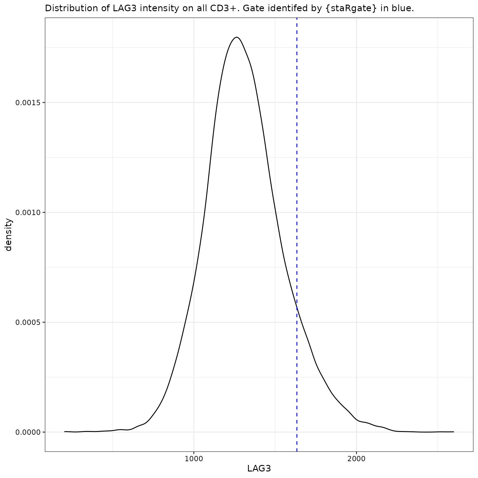

LAG3 by CD4 and CD8 subsets

# If by CD4/CD8,
intensity_dat |>
  dplyr::filter(cd3_pos == 1) |>
  # additional step to remove large intensity values only when density gating.
  # Still kept in the data
  dplyr::filter(!(dplyr::if_any(dplyr::all_of(markers_to_gate), ~ .x < neg_intensity_thres))) |>
  ggplot() +
  geom_density(aes(LAG3)) +
  geom_vline(
    data = dens_gates,
    aes(xintercept = LAG3),
    color = "blue",
    linetype = "dashed"
  ) +
  labs(subtitle = "Distribution of LAG3 intensity by CD4/CD8 subsets. Gate identifed by {staRgate} in blue.") +
  facet_wrap(~cd4_pos_cd8_pos)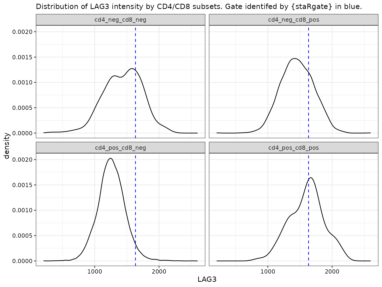

CCR7 for all CD3+

# For CCR7
intensity_dat |>
  dplyr::filter(cd3_pos == 1) |>
  # additional step to remove large intensity values only when density gating.
  # Still kept in the data
  dplyr::filter(!(dplyr::if_any(dplyr::all_of(markers_to_gate), ~ .x < neg_intensity_thres))) |>
  ggplot() +
  geom_density(aes(CCR7)) +
  geom_vline(
    data = dens_gates,
    aes(xintercept = CCR7),
    color = "blue",
    linetype = "dashed"
  ) +
  labs(subtitle = "Distribution of CCR7 intensity on all CD3+. Gate identifed by {staRgate} in blue.")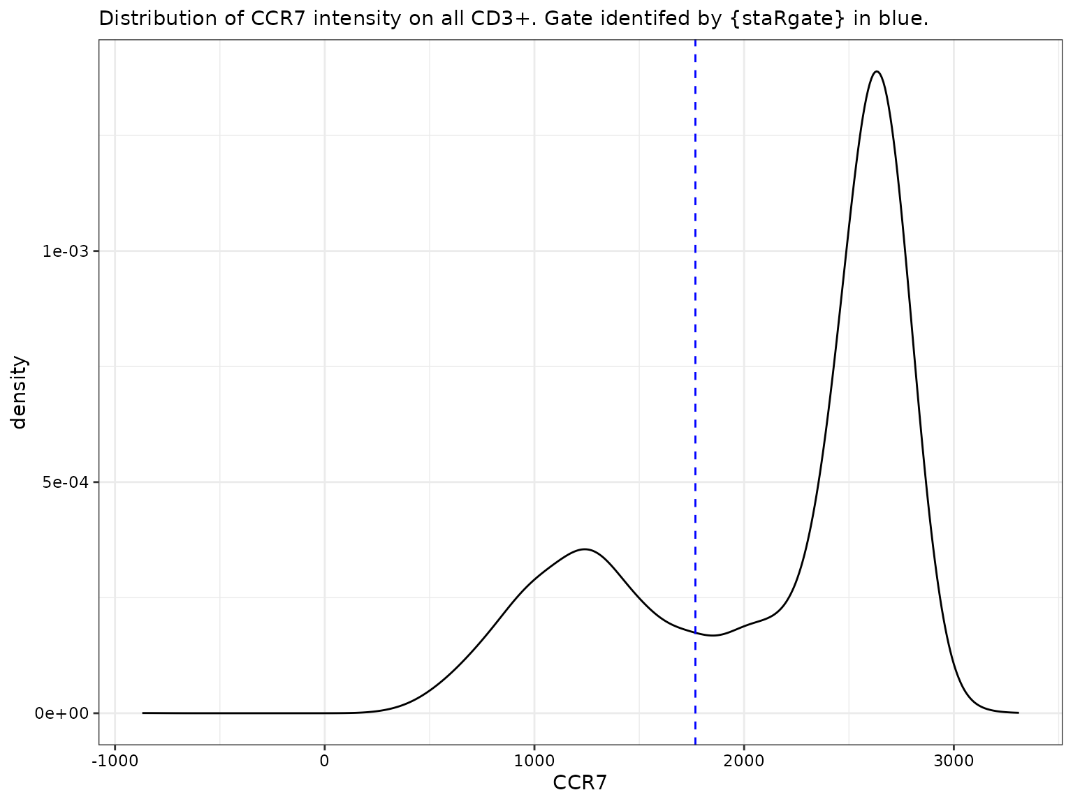

CCR7 by CD4 and CD8 subsets

# If by CD4/CD8,
intensity_dat |>
  dplyr::filter(cd3_pos == 1) |>
  # additional step to remove large intensity values only when density gating.
  # Still kept in the data
  dplyr::filter(!(dplyr::if_any(dplyr::all_of(markers_to_gate), ~ .x < neg_intensity_thres))) |>
  ggplot() +
  geom_density(aes(CCR7)) +
  geom_vline(
    data = dens_gates,
    aes(xintercept = CCR7),
    color = "blue",
    linetype = "dashed"
  ) +
  labs(subtitle = "Distribution of CCR7 intensity for CD4/CD8 subsets. Gate identifed by {staRgate} in blue.") +
  facet_wrap(~cd4_pos_cd8_pos)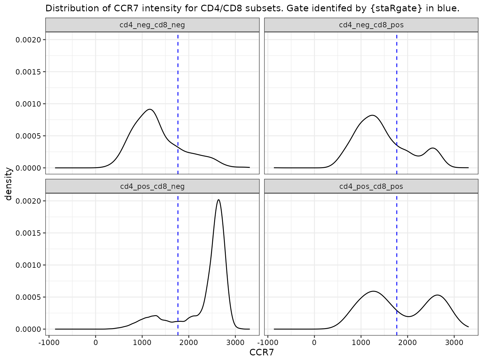

CD45RA for all CD3+

# For CD45RA
intensity_dat |>
  dplyr::filter(cd3_pos == 1) |>
  # additional step to remove large intensity values only when density gating.
  # Still kept in the data
  dplyr::filter(!(dplyr::if_any(dplyr::all_of(markers_to_gate), ~ .x < neg_intensity_thres))) |>
  ggplot() +
  geom_density(aes(CD45RA)) +
  geom_vline(
    data = dens_gates,
    aes(xintercept = CD45RA),
    color = "blue",
    linetype = "dashed"
  ) +
  labs(subtitle = "Distribution of CD45RA intensity on all CD3+. Gate identifed by {staRgate} in blue.")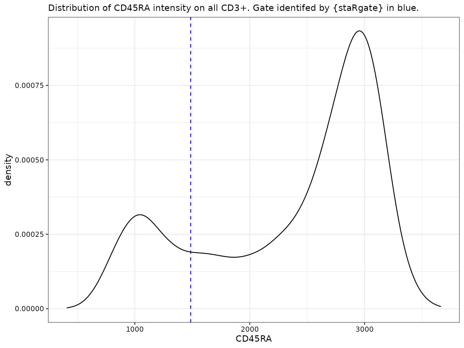

CD45RA by CD4 and CD8 subsets

# If by CD4/CD8,
intensity_dat |>
  dplyr::filter(cd3_pos == 1) |>
  # additional step to remove large intensity values only when density gating.
  # Still kept in the data
  dplyr::filter(!(dplyr::if_any(dplyr::all_of(markers_to_gate), ~ .x < neg_intensity_thres))) |>
  ggplot() +
  geom_density(aes(CD45RA)) +
  geom_vline(
    data = dens_gates,
    aes(xintercept = CD45RA),
    color = "blue",
    linetype = "dashed"
  ) +
  labs(subtitle = "Distribution of CD45RA intensity for CD4/CD8 subsets. Gate identifed by {staRgate} in blue.") +
  facet_wrap(~cd4_pos_cd8_pos)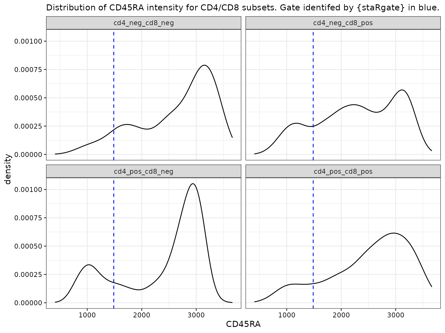

CD127 for all CD3+

# For CD127
intensity_dat |>
  dplyr::filter(cd3_pos == 1) |>
  # additional step to remove large intensity values only when density gating.
  # Still kept in the data
  dplyr::filter(!(dplyr::if_any(dplyr::all_of(markers_to_gate), ~ .x < neg_intensity_thres))) |>
  ggplot() +
  geom_density(aes(CD127)) +
  geom_vline(
    data = dens_gates,
    aes(xintercept = CD127),
    color = "blue",
    linetype = "dashed"
  ) +
  labs(subtitle = "Distribution of CD127 intensity on all CD3+. Gate identifed by {staRgate} in blue.")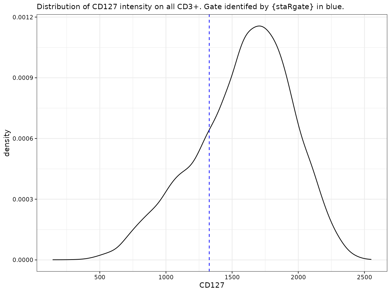

CD127 by CD4 and CD8 subsets

# If by CD4/CD8,
intensity_dat |>
  dplyr::filter(cd3_pos == 1) |>
  # additional step to remove large intensity values only when density gating.
  # Still kept in the data
  dplyr::filter(!(dplyr::if_any(dplyr::all_of(markers_to_gate), ~ .x < neg_intensity_thres))) |>
  ggplot() +
  geom_density(aes(CD127)) +
  geom_vline(
    data = dens_gates,
    aes(xintercept = CD127),
    color = "blue",
    linetype = "dashed"
  ) +
  labs(subtitle = "Distribution of CD127 intensity for CD4/CD8 subsets. Gate identifed by {staRgate} in blue.") +
  facet_wrap(~cd4_pos_cd8_pos)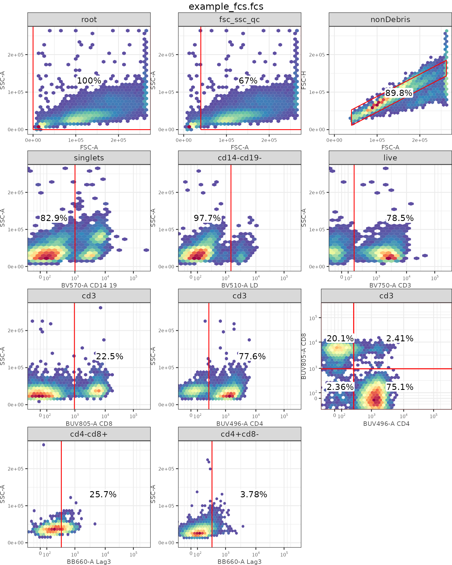

CD28 for all CD3+

# For CD28
intensity_dat |>
  dplyr::filter(cd3_pos == 1) |>
  # additional step to remove large intensity values only when density gating.
  # Still kept in the data
  dplyr::filter(!(dplyr::if_any(dplyr::all_of(markers_to_gate), ~ .x < neg_intensity_thres))) |>
  ggplot() +
  geom_density(aes(CD28)) +
  geom_vline(
    data = dens_gates,
    aes(xintercept = CD28),
    color = "blue",
    linetype = "dashed"
  ) +
  labs(subtitle = "Distribution of CD28 intensity on all CD3+. Gate identifed by {staRgate} in blue.")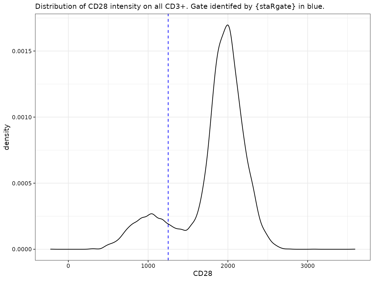

CD28 by CD4 and CD8 subsets

# If by CD4/CD8,
intensity_dat |>
  dplyr::filter(cd3_pos == 1) |>
  # additional step to remove large intensity values only when density gating.
  # Still kept in the data
  dplyr::filter(!(dplyr::if_any(dplyr::all_of(markers_to_gate), ~ .x < neg_intensity_thres))) |>
  ggplot() +
  geom_density(aes(CD28)) +
  geom_vline(
    data = dens_gates,
    aes(xintercept = CD28),
    color = "blue",
    linetype = "dashed"
  ) +
  labs(subtitle = "Distribution of CD28 intensity for CD4/CD8 subsets. Gate identifed by {staRgate} in blue.") +
  facet_wrap(~cd4_pos_cd8_pos)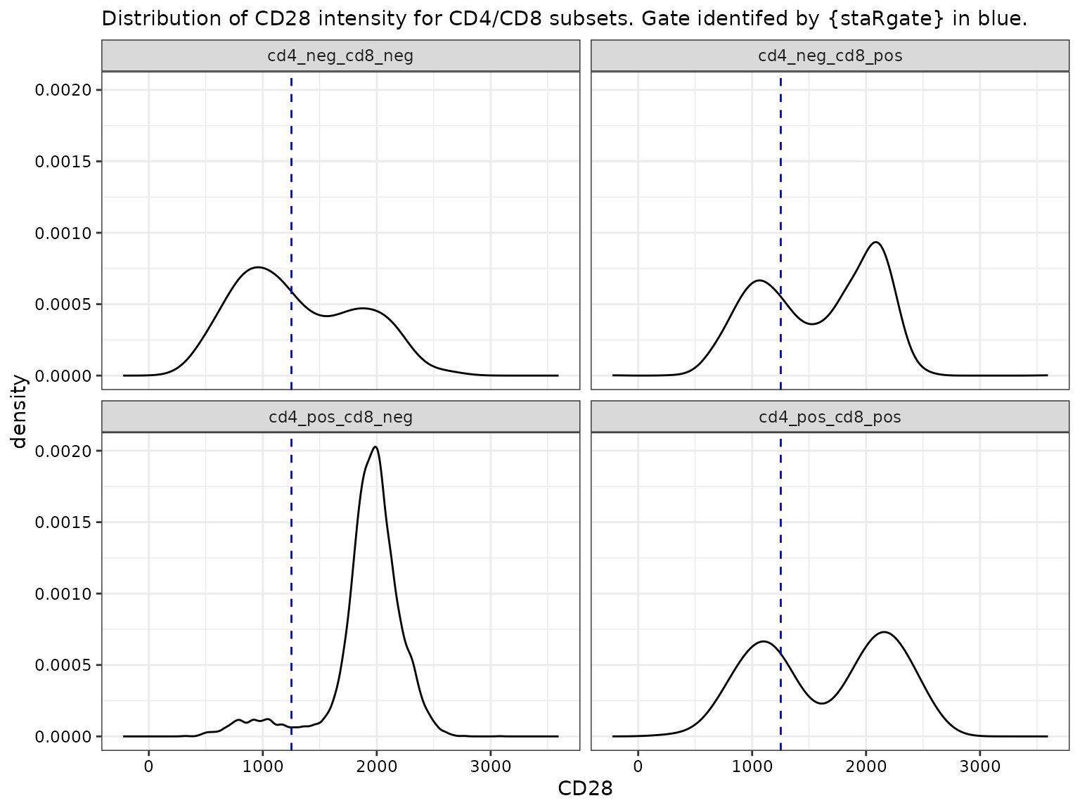

Getting percentage data

We can then summarize the single-cell level data to counts and percentages of cells for all combinations of markers.

For the subpopulations, the denominator is defined as the parent population and numerator is the population of interest out of the parent population. For example, the subpopulation CD4+ of CD3+ cells correspond to the CD4+ as the numerator and CD3+ as the denominator.

The $n_d$ refers to the number of markers considered for the denominator and $n$ for the number of markers considered for the numerator.

For the 29-marker panel, if the denominator is specified as the CD4 and CD8 subsets, then $n_d = 2$ and $n = 23$ for the markers of interest.

The getPerc function allows user to list the markers of interest for the numerator and denominator

In the example below, we will consider CD4 and CD8 subsets as the key parent populations of interest (denominator) and the three markers we gated on using c("LAG3", "CCR7", "CD45RA") (numerator markers).

The additional arguments expand_num and expand_denom generates different lists of subpopulations to calculate counts/percentages for:

expand_num: should calculations consider up to pairs of numerator markers included?,
expand_denom: should the calculations consider combinations of each numerator marker and parent populations specified in the denominator?

Currently, we support the four scenarios listed:

expand_num	expand_denom	The subpopulations to generate	Examples	Expected number of subpopulations¹	Expected number of subpopulations for the 29-marker T-cell panel
FALSE	FALSE	Numerator: Positive and negative for each marker specified Denominator: Combinations of positive and negative for markers specified	Numerator specified to (“LAG3”) and denominator specified as (“CD4”, “CD8”): LAG3+/- of CD4- & CD8- LAG3+/- of CD4+ & CD8- LAG3+/- of CD4+ & CD8+ LAG3+/- of CD4- & CD8+	2n*(2^n_d)	184
TRUE	FALSE	Numerator: Positive and negative for each marker specified, and combinations of positive/negative for pairs of markers At least 2 markers must be included in the numerator Denominator: Combinations of positive and negative for marker(s)	Numerator specified as (“LAG3”, “KI67”) and denominator as (“CD4”): LAG3+/- of CD4+/- KI67+/- of CD4+/- LAG3- KI67- of CD4+/- LAG3+ KI67- of CD4+/- LAG3- KI67+ of CD4+/- LAG3+ KI67+ of CD4+/-	2n(2^n_d) + 2^n_d(n choose 2)*(2²)	4232
FALSE	TRUE	Numerator: Positive and negative for each marker specified At least 2 markers must be included in the numerator Denominator: Combinations of positive and negative for marker(s), and combinations of positive and negative for marker(s) in denominator with one marker from the numerator	Numerator specified as (“LAG3”, “KI67”) and denominator as (“CD4”) LAG3+/- of CD4+/- KI67+/- of CD4+/- LAG3+/- of CD4-KI67- LAG3+/- of CD4-KI67+ LAG3+/- of CD4+KI67- LAG3+/- of CD4+KI67+ KI67+/- of CD4-LAG3- KI67+/- of CD4-LAG3+ KI67+/- of CD4+LAG3- KI67+/- of CD4+LAG3+	2n(2^n_d) + 42^n_dn(n-1)	8280
TRUE	TRUE	Numerator: Positive and negative for each marker specified, and combinations of positive/negative for pairs of markers At least 3 markers must be included in the numerator Denominator: Combinations of positive and negative for marker(s), and combinations of positive and negative for marker(s) in denominator with one marker from the numerator	Numerator specified as (“LAG3”, “KI67”, “CTLA4”) and denominator as (“CD4”) LAG3+/- of CD4+/- KI67+/- of CD4+/- CTLA4+/- of CD4+/- LAG3+/- of CD4-KI67- LAG3+/- of CD4-KI67+ LAG3+/- of CD4+KI67- LAG3+/- of CD4+KI67+ KI67+/- of CD4-LAG3- KI67+/- of CD4-LAG3+ KI67+/- of CD4+LAG3- KI67+/- of CD4+LAG3+ …. LAG3- KI67- of CD4+/- LAG3+ KI67- of CD4+/- LAG3- KI67+ of CD4+/- LAG3+ KI67+ of CD4+/- … LAG3+ KI67+ of CD4+/- & CTLA4+/- …	2n(2^n_d) + 2^n_d(n choose 2)(2²) + 42^n_dn(n-1) + 2²n((n-1) choose 2)*(2^n_d+1)	182344
¹ n, number of markers specified in the numerator; n_d, number of markers specified in the denominator

The keep_indicators argument provides the 0/1 for which marker is considered in the numerator and denominator for each subpopulation. This is especially useful when merging onto other data that does not have the same naming conventions.

For example, when matching strings: “CD4+ & CD8- of CD3+” is different from “CD8- & CD4+ of CD3+” and “CD4+ and CD8- of CD3+”. But using indicator columns, we can match the subpopulations regardless of the subpopulation naming convention.

Below is we show examples of each of the four combinations for the expand_num and expand_denom arguments.

For the example of when expand_num = FALSE and expand_denom = FALSE, keep_indicators = TRUE to illustrate the columns we get for the _POS and _POS_D. Other examples use keep_indicators = FALSE.

Expand example for expand_num = FALSE and expand_denom = FALSE, and keep_indicators = TRUE

example_perc1 <-
  # Should only count the CD3+ cells
  dplyr::filter(example_intensity_gated, cd3_pos == 1) |> 
  getPerc(
    intens_dat = _,
    num_marker = example_markers,
    denom_marker = c("CD4", "CD8"),
    expand_num = FALSE,
    expand_denom = FALSE,
    keep_indicators = TRUE
  )

# For display only, group based on the denominators and
# simplify the names to be numerators
example_perc1 |> 
  tidyr::separate_wider_delim(subpopulation,
    delim = "_OF_",
    names = c("num", "denom"),
    cols_remove = FALSE
  ) |>
  dplyr::mutate(denom = paste("Denom = ", denom)) |>
  dplyr::group_by(denom) |>
  dplyr::select(-subpopulation) |>
  gt::gt() |>
  gt::fmt_number(
    columns = "perc",
    decimals = 1
  )

num	n_num	n_denom	perc	LAG3_POS	CCR7_POS	CD45RA_POS	CD4_POS_D	CD8_POS_D
Denom = CD4_NEG_CD8_NEG
LAG3_NEG	196	271	72.3	0	NA	NA	0	0
CCR7_NEG	220	271	81.2	NA	0	NA	0	0
CD45RA_NEG	21	271	7.7	NA	NA	0	0	0
LAG3_POS	75	271	27.7	1	NA	NA	0	0
CCR7_POS	51	271	18.8	NA	1	NA	0	0
CD45RA_POS	250	271	92.3	NA	NA	1	0	0
Denom = CD4_NEG_CD8_POS
LAG3_NEG	1711	2302	74.3	0	NA	NA	0	1
CCR7_NEG	1699	2302	73.8	NA	0	NA	0	1
CD45RA_NEG	413	2302	17.9	NA	NA	0	0	1
LAG3_POS	591	2302	25.7	1	NA	NA	0	1
CCR7_POS	603	2302	26.2	NA	1	NA	0	1
CD45RA_POS	1889	2302	82.1	NA	NA	1	0	1
Denom = CD4_POS_CD8_NEG
LAG3_NEG	8289	8615	96.2	0	NA	NA	1	0
CCR7_NEG	1395	8615	16.2	NA	0	NA	1	0
CD45RA_NEG	1830	8615	21.2	NA	NA	0	1	0
LAG3_POS	326	8615	3.8	1	NA	NA	1	0
CCR7_POS	7220	8615	83.8	NA	1	NA	1	0
CD45RA_POS	6785	8615	78.8	NA	NA	1	1	0
Denom = CD4_POS_CD8_POS
LAG3_NEG	139	276	50.4	0	NA	NA	1	1
CCR7_NEG	152	276	55.1	NA	0	NA	1	1
CD45RA_NEG	35	276	12.7	NA	NA	0	1	1
LAG3_POS	137	276	49.6	1	NA	NA	1	1
CCR7_POS	124	276	44.9	NA	1	NA	1	1
CD45RA_POS	241	276	87.3	NA	NA	1	1	1

Expand example for expand_num = TRUE and expand_denom = FALSE, and keep_indicators = FALSE

example_perc2 <-
  # Should only count the CD3+ cells
  dplyr::filter(example_intensity_gated, cd3_pos == 1) |>
  getPerc(
    intens_dat = _,
    num_marker = example_markers,
    denom_marker = c("CD4", "CD8"),
    expand_num = TRUE,
    expand_denom = FALSE,
    keep_indicators = FALSE
  )

# For display only, group based on the denominators and
# simplify the names to be numerators
example_perc2 |>
  tidyr::separate_wider_delim(subpopulation,
    delim = "_OF_",
    names = c("num", "denom"),
    cols_remove = FALSE
  ) |>
  dplyr::mutate(denom = paste("Denom = ", denom)) |>
  dplyr::group_by(denom) |>
  dplyr::select(-subpopulation) |>
  gt::gt() |>
  gt::fmt_number(
    columns = "perc",
    decimals = 1
  )

num	n_num	n_denom	perc
Denom = CD4_NEG_CD8_NEG
LAG3_NEG	196	271	72.3
CCR7_NEG	220	271	81.2
CD45RA_NEG	21	271	7.7
LAG3_POS	75	271	27.7
CCR7_POS	51	271	18.8
CD45RA_POS	250	271	92.3
LAG3_NEG_CCR7_NEG	147	271	54.2
LAG3_NEG_CD45RA_NEG	17	271	6.3
LAG3_NEG_CCR7_POS	49	271	18.1
LAG3_NEG_CD45RA_POS	179	271	66.1
CCR7_NEG_CD45RA_NEG	17	271	6.3
CCR7_NEG_LAG3_POS	73	271	26.9
CCR7_NEG_CD45RA_POS	203	271	74.9
CD45RA_NEG_LAG3_POS	4	271	1.5
CD45RA_NEG_CCR7_POS	4	271	1.5
LAG3_POS_CCR7_POS	2	271	0.7
LAG3_POS_CD45RA_POS	71	271	26.2
CCR7_POS_CD45RA_POS	47	271	17.3
Denom = CD4_NEG_CD8_POS
LAG3_NEG	1711	2302	74.3
CCR7_NEG	1699	2302	73.8
CD45RA_NEG	413	2302	17.9
LAG3_POS	591	2302	25.7
CCR7_POS	603	2302	26.2
CD45RA_POS	1889	2302	82.1
LAG3_NEG_CCR7_NEG	1165	2302	50.6
LAG3_NEG_CD45RA_NEG	344	2302	14.9
LAG3_NEG_CCR7_POS	546	2302	23.7
LAG3_NEG_CD45RA_POS	1367	2302	59.4
CCR7_NEG_CD45RA_NEG	329	2302	14.3
CCR7_NEG_LAG3_POS	534	2302	23.2
CCR7_NEG_CD45RA_POS	1370	2302	59.5
CD45RA_NEG_LAG3_POS	69	2302	3.0
CD45RA_NEG_CCR7_POS	84	2302	3.6
LAG3_POS_CCR7_POS	57	2302	2.5
LAG3_POS_CD45RA_POS	522	2302	22.7
CCR7_POS_CD45RA_POS	519	2302	22.5
Denom = CD4_POS_CD8_NEG
LAG3_NEG	8289	8615	96.2
CCR7_NEG	1395	8615	16.2
CD45RA_NEG	1830	8615	21.2
LAG3_POS	326	8615	3.8
CCR7_POS	7220	8615	83.8
CD45RA_POS	6785	8615	78.8
LAG3_NEG_CCR7_NEG	1221	8615	14.2
LAG3_NEG_CD45RA_NEG	1700	8615	19.7
LAG3_NEG_CCR7_POS	7068	8615	82.0
LAG3_NEG_CD45RA_POS	6589	8615	76.5
CCR7_NEG_CD45RA_NEG	927	8615	10.8
CCR7_NEG_LAG3_POS	174	8615	2.0
CCR7_NEG_CD45RA_POS	468	8615	5.4
CD45RA_NEG_LAG3_POS	130	8615	1.5
CD45RA_NEG_CCR7_POS	903	8615	10.5
LAG3_POS_CCR7_POS	152	8615	1.8
LAG3_POS_CD45RA_POS	196	8615	2.3
CCR7_POS_CD45RA_POS	6317	8615	73.3
Denom = CD4_POS_CD8_POS
LAG3_NEG	139	276	50.4
CCR7_NEG	152	276	55.1
CD45RA_NEG	35	276	12.7
LAG3_POS	137	276	49.6
CCR7_POS	124	276	44.9
CD45RA_POS	241	276	87.3
LAG3_NEG_CCR7_NEG	79	276	28.6
LAG3_NEG_CD45RA_NEG	26	276	9.4
LAG3_NEG_CCR7_POS	60	276	21.7
LAG3_NEG_CD45RA_POS	113	276	40.9
CCR7_NEG_CD45RA_NEG	19	276	6.9
CCR7_NEG_LAG3_POS	73	276	26.4
CCR7_NEG_CD45RA_POS	133	276	48.2
CD45RA_NEG_LAG3_POS	9	276	3.3
CD45RA_NEG_CCR7_POS	16	276	5.8
LAG3_POS_CCR7_POS	64	276	23.2
LAG3_POS_CD45RA_POS	128	276	46.4
CCR7_POS_CD45RA_POS	108	276	39.1

Expand example for expand_num = FALSE and expand_denom = TRUE, and keep_indicators = FALSE

example_perc3 <-
  # Should only count the CD3+ cells
  dplyr::filter(example_intensity_gated, cd3_pos == 1) |>
  getPerc(
    intens_dat = _,
    num_marker = example_markers,
    denom_marker = c("CD4", "CD8"),
    expand_num = FALSE,
    expand_denom = TRUE,
    keep_indicators = FALSE
  )

# For display only, group based on the denominators and
# simplify the names to be numerators
example_perc3 |> 
  tidyr::separate_wider_delim(subpopulation,
    delim = "_OF_",
    names = c("num", "denom"),
    cols_remove = FALSE
  ) |>
  dplyr::mutate(denom = paste("Denom = ", denom)) |>
  dplyr::group_by(denom) |>
  dplyr::select(-subpopulation) |>
  gt::gt() |>
  gt::fmt_number(
    columns = "perc",
    decimals = 1
  )

num	n_num	n_denom	perc
Denom = CD4_NEG_CD8_NEG
LAG3_NEG	196	271	72.3
CCR7_NEG	220	271	81.2
CD45RA_NEG	21	271	7.7
LAG3_POS	75	271	27.7
CCR7_POS	51	271	18.8
CD45RA_POS	250	271	92.3
Denom = CD4_NEG_CD8_POS
LAG3_NEG	1711	2302	74.3
CCR7_NEG	1699	2302	73.8
CD45RA_NEG	413	2302	17.9
LAG3_POS	591	2302	25.7
CCR7_POS	603	2302	26.2
CD45RA_POS	1889	2302	82.1
Denom = CD4_POS_CD8_NEG
LAG3_NEG	8289	8615	96.2
CCR7_NEG	1395	8615	16.2
CD45RA_NEG	1830	8615	21.2
LAG3_POS	326	8615	3.8
CCR7_POS	7220	8615	83.8
CD45RA_POS	6785	8615	78.8
Denom = CD4_POS_CD8_POS
LAG3_NEG	139	276	50.4
CCR7_NEG	152	276	55.1
CD45RA_NEG	35	276	12.7
LAG3_POS	137	276	49.6
CCR7_POS	124	276	44.9
CD45RA_POS	241	276	87.3
Denom = CD4_NEG_CD8_NEG_LAG3_NEG
CCR7_NEG	147	196	75.0
CD45RA_NEG	17	196	8.7
CCR7_POS	49	196	25.0
CD45RA_POS	179	196	91.3
Denom = CD4_NEG_CD8_POS_LAG3_NEG
CCR7_NEG	1165	1711	68.1
CD45RA_NEG	344	1711	20.1
CCR7_POS	546	1711	31.9
CD45RA_POS	1367	1711	79.9
Denom = CD4_POS_CD8_NEG_LAG3_NEG
CCR7_NEG	1221	8289	14.7
CD45RA_NEG	1700	8289	20.5
CCR7_POS	7068	8289	85.3
CD45RA_POS	6589	8289	79.5
Denom = CD4_POS_CD8_POS_LAG3_NEG
CCR7_NEG	79	139	56.8
CD45RA_NEG	26	139	18.7
CCR7_POS	60	139	43.2
CD45RA_POS	113	139	81.3
Denom = CD4_NEG_CD8_NEG_CCR7_NEG
LAG3_NEG	147	220	66.8
CD45RA_NEG	17	220	7.7
LAG3_POS	73	220	33.2
CD45RA_POS	203	220	92.3
Denom = CD4_NEG_CD8_POS_CCR7_NEG
LAG3_NEG	1165	1699	68.6
CD45RA_NEG	329	1699	19.4
LAG3_POS	534	1699	31.4
CD45RA_POS	1370	1699	80.6
Denom = CD4_POS_CD8_NEG_CCR7_NEG
LAG3_NEG	1221	1395	87.5
CD45RA_NEG	927	1395	66.5
LAG3_POS	174	1395	12.5
CD45RA_POS	468	1395	33.5
Denom = CD4_POS_CD8_POS_CCR7_NEG
LAG3_NEG	79	152	52.0
CD45RA_NEG	19	152	12.5
LAG3_POS	73	152	48.0
CD45RA_POS	133	152	87.5
Denom = CD4_NEG_CD8_NEG_CD45RA_NEG
LAG3_NEG	17	21	81.0
CCR7_NEG	17	21	81.0
LAG3_POS	4	21	19.0
CCR7_POS	4	21	19.0
Denom = CD4_NEG_CD8_POS_CD45RA_NEG
LAG3_NEG	344	413	83.3
CCR7_NEG	329	413	79.7
LAG3_POS	69	413	16.7
CCR7_POS	84	413	20.3
Denom = CD4_POS_CD8_NEG_CD45RA_NEG
LAG3_NEG	1700	1830	92.9
CCR7_NEG	927	1830	50.7
LAG3_POS	130	1830	7.1
CCR7_POS	903	1830	49.3
Denom = CD4_POS_CD8_POS_CD45RA_NEG
LAG3_NEG	26	35	74.3
CCR7_NEG	19	35	54.3
LAG3_POS	9	35	25.7
CCR7_POS	16	35	45.7
Denom = CD4_NEG_CD8_NEG_LAG3_POS
CCR7_NEG	73	75	97.3
CD45RA_NEG	4	75	5.3
CCR7_POS	2	75	2.7
CD45RA_POS	71	75	94.7
Denom = CD4_NEG_CD8_POS_LAG3_POS
CCR7_NEG	534	591	90.4
CD45RA_NEG	69	591	11.7
CCR7_POS	57	591	9.6
CD45RA_POS	522	591	88.3
Denom = CD4_POS_CD8_NEG_LAG3_POS
CCR7_NEG	174	326	53.4
CD45RA_NEG	130	326	39.9
CCR7_POS	152	326	46.6
CD45RA_POS	196	326	60.1
Denom = CD4_POS_CD8_POS_LAG3_POS
CCR7_NEG	73	137	53.3
CD45RA_NEG	9	137	6.6
CCR7_POS	64	137	46.7
CD45RA_POS	128	137	93.4
Denom = CD4_NEG_CD8_NEG_CCR7_POS
LAG3_NEG	49	51	96.1
CD45RA_NEG	4	51	7.8
LAG3_POS	2	51	3.9
CD45RA_POS	47	51	92.2
Denom = CD4_NEG_CD8_POS_CCR7_POS
LAG3_NEG	546	603	90.5
CD45RA_NEG	84	603	13.9
LAG3_POS	57	603	9.5
CD45RA_POS	519	603	86.1
Denom = CD4_POS_CD8_NEG_CCR7_POS
LAG3_NEG	7068	7220	97.9
CD45RA_NEG	903	7220	12.5
LAG3_POS	152	7220	2.1
CD45RA_POS	6317	7220	87.5
Denom = CD4_POS_CD8_POS_CCR7_POS
LAG3_NEG	60	124	48.4
CD45RA_NEG	16	124	12.9
LAG3_POS	64	124	51.6
CD45RA_POS	108	124	87.1
Denom = CD4_NEG_CD8_NEG_CD45RA_POS
LAG3_NEG	179	250	71.6
CCR7_NEG	203	250	81.2
LAG3_POS	71	250	28.4
CCR7_POS	47	250	18.8
Denom = CD4_NEG_CD8_POS_CD45RA_POS
LAG3_NEG	1367	1889	72.4
CCR7_NEG	1370	1889	72.5
LAG3_POS	522	1889	27.6
CCR7_POS	519	1889	27.5
Denom = CD4_POS_CD8_NEG_CD45RA_POS
LAG3_NEG	6589	6785	97.1
CCR7_NEG	468	6785	6.9
LAG3_POS	196	6785	2.9
CCR7_POS	6317	6785	93.1
Denom = CD4_POS_CD8_POS_CD45RA_POS
LAG3_NEG	113	241	46.9
CCR7_NEG	133	241	55.2
LAG3_POS	128	241	53.1
CCR7_POS	108	241	44.8

Expand example for expand_num = TRUE and expand_denom = TRUE , and keep_indicators = FALSE

example_perc4 <-
  # Should only count the CD3+ cells
  dplyr::filter(example_intensity_gated, cd3_pos == 1) |>
  getPerc(
    intens_dat = _,
    num_marker = example_markers,
    denom_marker = c("CD4", "CD8"),
    expand_num = TRUE,
    expand_denom = TRUE,
    keep_indicators = FALSE
  )

# For display only, group based on the denominators and
# simplify the names to be numerators
example_perc4 |>
  tidyr::separate_wider_delim(subpopulation,
    delim = "_OF_",
    names = c("num", "denom"),
    cols_remove = FALSE
  ) |>
  dplyr::mutate(denom = paste("Denom = ", denom)) |>
  dplyr::group_by(denom) |>
  dplyr::select(-subpopulation) |>
  gt::gt() |>
  gt::fmt_number(
    columns = "perc",
    decimals = 1
  )

num	n_num	n_denom	perc
Denom = CD4_NEG_CD8_NEG
LAG3_NEG	196	271	72.3
CCR7_NEG	220	271	81.2
CD45RA_NEG	21	271	7.7
LAG3_POS	75	271	27.7
CCR7_POS	51	271	18.8
CD45RA_POS	250	271	92.3
LAG3_NEG_CCR7_NEG	147	271	54.2
LAG3_NEG_CD45RA_NEG	17	271	6.3
LAG3_NEG_CCR7_POS	49	271	18.1
LAG3_NEG_CD45RA_POS	179	271	66.1
CCR7_NEG_CD45RA_NEG	17	271	6.3
CCR7_NEG_LAG3_POS	73	271	26.9
CCR7_NEG_CD45RA_POS	203	271	74.9
CD45RA_NEG_LAG3_POS	4	271	1.5
CD45RA_NEG_CCR7_POS	4	271	1.5
LAG3_POS_CCR7_POS	2	271	0.7
LAG3_POS_CD45RA_POS	71	271	26.2
CCR7_POS_CD45RA_POS	47	271	17.3
Denom = CD4_NEG_CD8_POS
LAG3_NEG	1711	2302	74.3
CCR7_NEG	1699	2302	73.8
CD45RA_NEG	413	2302	17.9
LAG3_POS	591	2302	25.7
CCR7_POS	603	2302	26.2
CD45RA_POS	1889	2302	82.1
LAG3_NEG_CCR7_NEG	1165	2302	50.6
LAG3_NEG_CD45RA_NEG	344	2302	14.9
LAG3_NEG_CCR7_POS	546	2302	23.7
LAG3_NEG_CD45RA_POS	1367	2302	59.4
CCR7_NEG_CD45RA_NEG	329	2302	14.3
CCR7_NEG_LAG3_POS	534	2302	23.2
CCR7_NEG_CD45RA_POS	1370	2302	59.5
CD45RA_NEG_LAG3_POS	69	2302	3.0
CD45RA_NEG_CCR7_POS	84	2302	3.6
LAG3_POS_CCR7_POS	57	2302	2.5
LAG3_POS_CD45RA_POS	522	2302	22.7
CCR7_POS_CD45RA_POS	519	2302	22.5
Denom = CD4_POS_CD8_NEG
LAG3_NEG	8289	8615	96.2
CCR7_NEG	1395	8615	16.2
CD45RA_NEG	1830	8615	21.2
LAG3_POS	326	8615	3.8
CCR7_POS	7220	8615	83.8
CD45RA_POS	6785	8615	78.8
LAG3_NEG_CCR7_NEG	1221	8615	14.2
LAG3_NEG_CD45RA_NEG	1700	8615	19.7
LAG3_NEG_CCR7_POS	7068	8615	82.0
LAG3_NEG_CD45RA_POS	6589	8615	76.5
CCR7_NEG_CD45RA_NEG	927	8615	10.8
CCR7_NEG_LAG3_POS	174	8615	2.0
CCR7_NEG_CD45RA_POS	468	8615	5.4
CD45RA_NEG_LAG3_POS	130	8615	1.5
CD45RA_NEG_CCR7_POS	903	8615	10.5
LAG3_POS_CCR7_POS	152	8615	1.8
LAG3_POS_CD45RA_POS	196	8615	2.3
CCR7_POS_CD45RA_POS	6317	8615	73.3
Denom = CD4_POS_CD8_POS
LAG3_NEG	139	276	50.4
CCR7_NEG	152	276	55.1
CD45RA_NEG	35	276	12.7
LAG3_POS	137	276	49.6
CCR7_POS	124	276	44.9
CD45RA_POS	241	276	87.3
LAG3_NEG_CCR7_NEG	79	276	28.6
LAG3_NEG_CD45RA_NEG	26	276	9.4
LAG3_NEG_CCR7_POS	60	276	21.7
LAG3_NEG_CD45RA_POS	113	276	40.9
CCR7_NEG_CD45RA_NEG	19	276	6.9
CCR7_NEG_LAG3_POS	73	276	26.4
CCR7_NEG_CD45RA_POS	133	276	48.2
CD45RA_NEG_LAG3_POS	9	276	3.3
CD45RA_NEG_CCR7_POS	16	276	5.8
LAG3_POS_CCR7_POS	64	276	23.2
LAG3_POS_CD45RA_POS	128	276	46.4
CCR7_POS_CD45RA_POS	108	276	39.1
Denom = CD4_NEG_CD8_NEG_LAG3_NEG
CCR7_NEG	147	196	75.0
CD45RA_NEG	17	196	8.7
CCR7_POS	49	196	25.0
CD45RA_POS	179	196	91.3
CCR7_NEG_CD45RA_NEG	15	196	7.7
CCR7_NEG_CD45RA_POS	132	196	67.3
CD45RA_NEG_CCR7_POS	2	196	1.0
CCR7_POS_CD45RA_POS	47	196	24.0
Denom = CD4_NEG_CD8_POS_LAG3_NEG
CCR7_NEG	1165	1711	68.1
CD45RA_NEG	344	1711	20.1
CCR7_POS	546	1711	31.9
CD45RA_POS	1367	1711	79.9
CCR7_NEG_CD45RA_NEG	269	1711	15.7
CCR7_NEG_CD45RA_POS	896	1711	52.4
CD45RA_NEG_CCR7_POS	75	1711	4.4
CCR7_POS_CD45RA_POS	471	1711	27.5
Denom = CD4_POS_CD8_NEG_LAG3_NEG
CCR7_NEG	1221	8289	14.7
CD45RA_NEG	1700	8289	20.5
CCR7_POS	7068	8289	85.3
CD45RA_POS	6589	8289	79.5
CCR7_NEG_CD45RA_NEG	837	8289	10.1
CCR7_NEG_CD45RA_POS	384	8289	4.6
CD45RA_NEG_CCR7_POS	863	8289	10.4
CCR7_POS_CD45RA_POS	6205	8289	74.9
Denom = CD4_POS_CD8_POS_LAG3_NEG
CCR7_NEG	79	139	56.8
CD45RA_NEG	26	139	18.7
CCR7_POS	60	139	43.2
CD45RA_POS	113	139	81.3
CCR7_NEG_CD45RA_NEG	11	139	7.9
CCR7_NEG_CD45RA_POS	68	139	48.9
CD45RA_NEG_CCR7_POS	15	139	10.8
CCR7_POS_CD45RA_POS	45	139	32.4
Denom = CD4_NEG_CD8_NEG_CCR7_NEG
LAG3_NEG	147	220	66.8
CD45RA_NEG	17	220	7.7
LAG3_POS	73	220	33.2
CD45RA_POS	203	220	92.3
LAG3_NEG_CD45RA_NEG	15	220	6.8
LAG3_NEG_CD45RA_POS	132	220	60.0
CD45RA_NEG_LAG3_POS	2	220	0.9
LAG3_POS_CD45RA_POS	71	220	32.3
Denom = CD4_NEG_CD8_POS_CCR7_NEG
LAG3_NEG	1165	1699	68.6
CD45RA_NEG	329	1699	19.4
LAG3_POS	534	1699	31.4
CD45RA_POS	1370	1699	80.6
LAG3_NEG_CD45RA_NEG	269	1699	15.8
LAG3_NEG_CD45RA_POS	896	1699	52.7
CD45RA_NEG_LAG3_POS	60	1699	3.5
LAG3_POS_CD45RA_POS	474	1699	27.9
Denom = CD4_POS_CD8_NEG_CCR7_NEG
LAG3_NEG	1221	1395	87.5
CD45RA_NEG	927	1395	66.5
LAG3_POS	174	1395	12.5
CD45RA_POS	468	1395	33.5
LAG3_NEG_CD45RA_NEG	837	1395	60.0
LAG3_NEG_CD45RA_POS	384	1395	27.5
CD45RA_NEG_LAG3_POS	90	1395	6.5
LAG3_POS_CD45RA_POS	84	1395	6.0
Denom = CD4_POS_CD8_POS_CCR7_NEG
LAG3_NEG	79	152	52.0
CD45RA_NEG	19	152	12.5
LAG3_POS	73	152	48.0
CD45RA_POS	133	152	87.5
LAG3_NEG_CD45RA_NEG	11	152	7.2
LAG3_NEG_CD45RA_POS	68	152	44.7
CD45RA_NEG_LAG3_POS	8	152	5.3
LAG3_POS_CD45RA_POS	65	152	42.8
Denom = CD4_NEG_CD8_NEG_CD45RA_NEG
LAG3_NEG	17	21	81.0
CCR7_NEG	17	21	81.0
LAG3_POS	4	21	19.0
CCR7_POS	4	21	19.0
LAG3_NEG_CCR7_NEG	15	21	71.4
LAG3_NEG_CCR7_POS	2	21	9.5
CCR7_NEG_LAG3_POS	2	21	9.5
LAG3_POS_CCR7_POS	2	21	9.5
Denom = CD4_NEG_CD8_POS_CD45RA_NEG
LAG3_NEG	344	413	83.3
CCR7_NEG	329	413	79.7
LAG3_POS	69	413	16.7
CCR7_POS	84	413	20.3
LAG3_NEG_CCR7_NEG	269	413	65.1
LAG3_NEG_CCR7_POS	75	413	18.2
CCR7_NEG_LAG3_POS	60	413	14.5
LAG3_POS_CCR7_POS	9	413	2.2
Denom = CD4_POS_CD8_NEG_CD45RA_NEG
LAG3_NEG	1700	1830	92.9
CCR7_NEG	927	1830	50.7
LAG3_POS	130	1830	7.1
CCR7_POS	903	1830	49.3
LAG3_NEG_CCR7_NEG	837	1830	45.7
LAG3_NEG_CCR7_POS	863	1830	47.2
CCR7_NEG_LAG3_POS	90	1830	4.9
LAG3_POS_CCR7_POS	40	1830	2.2
Denom = CD4_POS_CD8_POS_CD45RA_NEG
LAG3_NEG	26	35	74.3
CCR7_NEG	19	35	54.3
LAG3_POS	9	35	25.7
CCR7_POS	16	35	45.7
LAG3_NEG_CCR7_NEG	11	35	31.4
LAG3_NEG_CCR7_POS	15	35	42.9
CCR7_NEG_LAG3_POS	8	35	22.9
LAG3_POS_CCR7_POS	1	35	2.9
Denom = CD4_NEG_CD8_NEG_LAG3_POS
CCR7_NEG	73	75	97.3
CD45RA_NEG	4	75	5.3
CCR7_POS	2	75	2.7
CD45RA_POS	71	75	94.7
CCR7_NEG_CD45RA_NEG	2	75	2.7
CCR7_NEG_CD45RA_POS	71	75	94.7
CD45RA_NEG_CCR7_POS	2	75	2.7
CCR7_POS_CD45RA_POS	0	75	0.0
Denom = CD4_NEG_CD8_POS_LAG3_POS
CCR7_NEG	534	591	90.4
CD45RA_NEG	69	591	11.7
CCR7_POS	57	591	9.6
CD45RA_POS	522	591	88.3
CCR7_NEG_CD45RA_NEG	60	591	10.2
CCR7_NEG_CD45RA_POS	474	591	80.2
CD45RA_NEG_CCR7_POS	9	591	1.5
CCR7_POS_CD45RA_POS	48	591	8.1
Denom = CD4_POS_CD8_NEG_LAG3_POS
CCR7_NEG	174	326	53.4
CD45RA_NEG	130	326	39.9
CCR7_POS	152	326	46.6
CD45RA_POS	196	326	60.1
CCR7_NEG_CD45RA_NEG	90	326	27.6
CCR7_NEG_CD45RA_POS	84	326	25.8
CD45RA_NEG_CCR7_POS	40	326	12.3
CCR7_POS_CD45RA_POS	112	326	34.4
Denom = CD4_POS_CD8_POS_LAG3_POS
CCR7_NEG	73	137	53.3
CD45RA_NEG	9	137	6.6
CCR7_POS	64	137	46.7
CD45RA_POS	128	137	93.4
CCR7_NEG_CD45RA_NEG	8	137	5.8
CCR7_NEG_CD45RA_POS	65	137	47.4
CD45RA_NEG_CCR7_POS	1	137	0.7
CCR7_POS_CD45RA_POS	63	137	46.0
Denom = CD4_NEG_CD8_NEG_CCR7_POS
LAG3_NEG	49	51	96.1
CD45RA_NEG	4	51	7.8
LAG3_POS	2	51	3.9
CD45RA_POS	47	51	92.2
LAG3_NEG_CD45RA_NEG	2	51	3.9
LAG3_NEG_CD45RA_POS	47	51	92.2
CD45RA_NEG_LAG3_POS	2	51	3.9
LAG3_POS_CD45RA_POS	0	51	0.0
Denom = CD4_NEG_CD8_POS_CCR7_POS
LAG3_NEG	546	603	90.5
CD45RA_NEG	84	603	13.9
LAG3_POS	57	603	9.5
CD45RA_POS	519	603	86.1
LAG3_NEG_CD45RA_NEG	75	603	12.4
LAG3_NEG_CD45RA_POS	471	603	78.1
CD45RA_NEG_LAG3_POS	9	603	1.5
LAG3_POS_CD45RA_POS	48	603	8.0
Denom = CD4_POS_CD8_NEG_CCR7_POS
LAG3_NEG	7068	7220	97.9
CD45RA_NEG	903	7220	12.5
LAG3_POS	152	7220	2.1
CD45RA_POS	6317	7220	87.5
LAG3_NEG_CD45RA_NEG	863	7220	12.0
LAG3_NEG_CD45RA_POS	6205	7220	85.9
CD45RA_NEG_LAG3_POS	40	7220	0.6
LAG3_POS_CD45RA_POS	112	7220	1.6
Denom = CD4_POS_CD8_POS_CCR7_POS
LAG3_NEG	60	124	48.4
CD45RA_NEG	16	124	12.9
LAG3_POS	64	124	51.6
CD45RA_POS	108	124	87.1
LAG3_NEG_CD45RA_NEG	15	124	12.1
LAG3_NEG_CD45RA_POS	45	124	36.3
CD45RA_NEG_LAG3_POS	1	124	0.8
LAG3_POS_CD45RA_POS	63	124	50.8
Denom = CD4_NEG_CD8_NEG_CD45RA_POS
LAG3_NEG	179	250	71.6
CCR7_NEG	203	250	81.2
LAG3_POS	71	250	28.4
CCR7_POS	47	250	18.8
LAG3_NEG_CCR7_NEG	132	250	52.8
LAG3_NEG_CCR7_POS	47	250	18.8
CCR7_NEG_LAG3_POS	71	250	28.4
LAG3_POS_CCR7_POS	0	250	0.0
Denom = CD4_NEG_CD8_POS_CD45RA_POS
LAG3_NEG	1367	1889	72.4
CCR7_NEG	1370	1889	72.5
LAG3_POS	522	1889	27.6
CCR7_POS	519	1889	27.5
LAG3_NEG_CCR7_NEG	896	1889	47.4
LAG3_NEG_CCR7_POS	471	1889	24.9
CCR7_NEG_LAG3_POS	474	1889	25.1
LAG3_POS_CCR7_POS	48	1889	2.5
Denom = CD4_POS_CD8_NEG_CD45RA_POS
LAG3_NEG	6589	6785	97.1
CCR7_NEG	468	6785	6.9
LAG3_POS	196	6785	2.9
CCR7_POS	6317	6785	93.1
LAG3_NEG_CCR7_NEG	384	6785	5.7
LAG3_NEG_CCR7_POS	6205	6785	91.5
CCR7_NEG_LAG3_POS	84	6785	1.2
LAG3_POS_CCR7_POS	112	6785	1.7
Denom = CD4_POS_CD8_POS_CD45RA_POS
LAG3_NEG	113	241	46.9
CCR7_NEG	133	241	55.2
LAG3_POS	128	241	53.1
CCR7_POS	108	241	44.8
LAG3_NEG_CCR7_NEG	68	241	28.2
LAG3_NEG_CCR7_POS	45	241	18.7
CCR7_NEG_LAG3_POS	65	241	27.0
LAG3_POS_CCR7_POS	63	241	26.1

Optional: Adding density gates back to GatingSet

Let’s add the gate for LAG3 of CD4+ and CD8+. This is a good visualization to see all sequential gating steps applied to the sample.

# Grab gate as a numeric
current_gate <-
  dens_gates |>
  dplyr::filter(cd4_pos_cd8_pos == "cd4_neg_cd8_pos") |>
  dplyr::pull(LAG3)

# Apply using gs_add_gating-method and
# We want a boundary gate
openCyto::gs_add_gating_method(
  gs,
  alias = "lag3_cd8",
  pop = "+",
  parent = "cd4-cd8+",
  dims = "LAG3",
  gating_method = "boundary",
  gating_args = list(min = current_gate, max = Inf)
)

current_gate <-
  dens_gates |>
  dplyr::filter(cd4_pos_cd8_pos == "cd4_pos_cd8_neg") |>
  dplyr::pull(LAG3)

openCyto::gs_add_gating_method(
  gs,
  alias = "lag3_cd4",
  pop = "+",
  parent = "cd4+cd8-",
  dims = "LAG3",
  gating_method = "boundary",
  gating_args = list(min = current_gate, max = Inf)
)

ggcyto::autoplot(gs[[1]])

After running {staRgate} to gate flow cytometry data, it is recommended to perform some quality checks (QC) on the gate placements to ensure they are reasonable. We suggest to use ridgeplots in addition to the ggcyto::autoplot function to visualize the density distributions per marker across samples. When examining a large batch of samples, downsampling, such as to a random sample of 10k CD3+ cells, will make the QC process more manageable. In addition, random spot checks of a few samples would also be helpful QC to detect any edge cases.

Currently in this tutorial, we do not extend to the QC steps and suggest to lean on other examples for how to put together a ridgeplot for example.

In the near future, we hope to incorporate some examples for the additional QC steps as well, stay tuned!

Session info

sessionInfo()
#> R version 4.5.2 (2025-10-31)
#> Platform: x86_64-pc-linux-gnu
#> Running under: Ubuntu 24.04.3 LTS
#> 
#> Matrix products: default
#> BLAS:   /usr/lib/x86_64-linux-gnu/openblas-pthread/libblas.so.3 
#> LAPACK: /usr/lib/x86_64-linux-gnu/openblas-pthread/libopenblasp-r0.3.26.so;  LAPACK version 3.12.0
#> 
#> locale:
#>  [1] LC_CTYPE=C.UTF-8       LC_NUMERIC=C           LC_TIME=C.UTF-8       
#>  [4] LC_COLLATE=C.UTF-8     LC_MONETARY=C.UTF-8    LC_MESSAGES=C.UTF-8   
#>  [7] LC_PAPER=C.UTF-8       LC_NAME=C              LC_ADDRESS=C          
#> [10] LC_TELEPHONE=C         LC_MEASUREMENT=C.UTF-8 LC_IDENTIFICATION=C   
#> 
#> time zone: UTC
#> tzcode source: system (glibc)
#> 
#> attached base packages:
#> [1] stats     graphics  grDevices utils     datasets  methods   base     
#> 
#> other attached packages:
#> [1] ggcyto_1.38.0        ncdfFlow_2.56.0      BH_1.87.0-1         
#> [4] ggplot2_4.0.1        flowCore_2.22.0      flowWorkspace_4.22.0
#> [7] openCyto_2.22.0      staRgate_0.99.4      BiocStyle_2.38.0    
#> 
#> loaded via a namespace (and not attached):
#>  [1] gtable_0.3.6        xfun_0.54           bslib_0.9.0        
#>  [4] htmlwidgets_1.6.4   Biobase_2.70.0      lattice_0.22-7     
#>  [7] vctrs_0.6.5         tools_4.5.2         generics_0.1.4     
#> [10] stats4_4.5.2        parallel_4.5.2      tibble_3.3.0       
#> [13] pkgconfig_2.0.3     data.table_1.17.8   RColorBrewer_1.1-3 
#> [16] S7_0.2.1            desc_1.4.3          S4Vectors_0.48.0   
#> [19] gt_1.1.0            graph_1.88.0        lifecycle_1.0.4    
#> [22] compiler_4.5.2      farver_2.1.2        stringr_1.6.0      
#> [25] textshaping_1.0.4   janitor_2.2.1       snakecase_0.11.1   
#> [28] litedown_0.8        htmltools_0.5.8.1   sass_0.4.10        
#> [31] yaml_2.3.10         pillar_1.11.1       pkgdown_2.2.0      
#> [34] hexbin_1.28.5       jquerylib_0.1.4     tidyr_1.3.1        
#> [37] cachem_1.1.0        RProtoBufLib_2.22.0 commonmark_2.0.0   
#> [40] tidyselect_1.2.1    digest_0.6.38       stringi_1.8.7      
#> [43] dplyr_1.1.4         purrr_1.2.0         bookdown_0.45      
#> [46] labeling_0.4.3      flowClust_3.48.0    fastmap_1.2.0      
#> [49] grid_4.5.2          cli_3.6.5           magrittr_2.0.4     
#> [52] utf8_1.2.6          RBGL_1.86.0         XML_3.99-0.20      
#> [55] withr_3.0.2         scales_1.4.0        timechange_0.3.0   
#> [58] lubridate_1.9.4     rmarkdown_2.30      matrixStats_1.5.0  
#> [61] gridExtra_2.3       cytolib_2.22.0      ragg_1.5.0         
#> [64] evaluate_1.0.5      knitr_1.50          markdown_2.0       
#> [67] rlang_1.1.6         Rcpp_1.1.0          glue_1.8.0         
#> [70] xml2_1.5.0          Rgraphviz_2.54.0    BiocManager_1.30.27
#> [73] BiocGenerics_0.56.0 jsonlite_2.0.0      R6_2.6.1           
#> [76] plyr_1.8.9          systemfonts_1.3.1   fs_1.6.6

References

G. Finak, J. Frelinger, W. Jiang, E. W. Newell, J. Ramey, M. M. Davis, S. A. Kalams, S. C. De Rosa and R. Gottardo, “OpenCyto: An Open Source Infrastructure for Scalable, Robust, Reproducible, and Automated, End-to-End Flow Cytometry Data Analysis,” PLoS Computational Biology, vol. 10, p. e1003806, August 2014.

G. Finak and M. Jiang, “flowWorkspace: Infrastructure for representing and interacting with gated and ungated cytometry data sets.,” 2023.

G. Finak, W. Jiang and R. Gottardo, “CytoML for cross-platform cytometry data sharing,” Cytometry Part A, vol. 93, pp. -7, 2018.

G. Monaco, H. Chen, M. Poidinger, J. Chen, J. P. de Magalhães and A. Larbi, “flowAI: automatic and interactive anomaly discerning tools for flow cytometry data,” Bioinformatics, vol. 32, p. 2473–2480, April 2016. P. Van, W. Jiang, R. Gottardo and G. Finak, “ggcyto: Next-generation open-source visualization software for cytometry,” Bioinformatics, 2018.